Sex Determination and X chromosome contamination estimate
One way to determine the nuclear contamination estimate works only in male samples. It is based on the fact that males have only one copy of the X chromosome, so any detectable heterozygosity on the X chromosome in males would suggest certain amount of contamination. Note that the sex of the contaminating sample is not important here, as both male and female contamination would contribute at least one more x chromosome, which would show up in this contamination test.
We will proceed in two steps. First, we need to determine the molecular sex of each sample. Second, we will run ANGSD for contamination estimation on all male samples.
Sex determination
On the cluster
The basic idea here is to compare genomic coverage on the X chromosome with the genomic coverage on autosomal chromosomes. Since males have only one copy of the X, coverage on X should be half the value on autosomes, while in females it should be roughly the same. Similarly, since males one copy of Y, coverage on Y should be half the value of autosomes in males, and it should be zero in females.
The first step is to run samtools depth on the bam files. To get an idea on what this tool does, first run it and look at the first 10 lines only:
samtools depth -q30 -Q37 -a -b $SNP_POS $BAM_FILE | head
Generally, when I write $SNP_POS or $BAM_FILE, you need to replace those variables with actual file names. Here, -b $SNP_POS inputs a text file that contains the positions in the capture experiment. We have prepared various SNP positions files for you, for both 390K and 1240K capture panels. You can find them in /projects1/Reference_Genomes/Human/hs37d5/SNPCapBEDs and /projects1/Reference_Genomes/Human/HG19/SNPCapBEDs, depending on which reference genome you have used to map the genome you are working with, and which SNP panel was used (e.g. 1240k). The flags -q30 -Q37 are filters on base- and mapping quality, and the -a flag forces output of every site, even those with coverage 0 (which is important for counting sites). Finally, $BAM_FILE denotes the - wait for it - bam file.
The output of this command should look like this:
1   752567  0
1   776546  1
1   832918  0
1   842013  0
1   846864  0
1   869303  0
1   891021  5
1   896271  0
1   903427  0
1   912660  1
(Use Ctrl-C to stop the command if it stalls.) The columns denote chromosome, position and the number of reads covering that site. We now need to write a little script that counts those read numbers for us, distinguishing autosomes, X chromosome and Y chromosome. Here is my version of this in awk:
BEGIN {
    xReads = 0
    yReads = 0
    autReads = 0

    xSites = 0
    ySites = 0
    autSites = 0
}
{
    chr = $1
    pos = $2
    cov = $3
    if(chr == "chrX") {
        xReads += cov
        xSites += 1
    }
    else if(chr == "chrY") {
        yReads += cov
        ySites += 1
    }
    else {
        autReads += cov
        autSites += 1
    }
}
END {
    OFS="\t"
    print("xCoverage", xSites > 0 ? xReads / xSites : 0)
    print("yCoverage", ySites > 0 ? yReads / ySites : 0)
    print("autCoverage", autSites > 0 ? autReads / autSites : 0)
}
awk is a very useful UNIX utility that is perfect for doing simple counting- or other statistics on file streams. You can learn awk yourself if you want, but for now the only important thing are the code lines which read
if(chr == "X") {
    ...
}
else if(chr == "Y") {
    ...
}
else {
    ...
}
As you can see, these lines check whether the chromosome is X or Y or neither of them (autosomes). Here you need to make sure that the names of the chromosomes are the same as in the reference that you used to align the sequences. You can quickly check that from the output of the samtools depth command above. If the first column looks like chr1 or chr2 instead of 1 or 2, than you need to change the awk script lines above to:
if(chr == "chrX") {
    ...
}
else if(chr == "chrY") {
    ...
}
else {
    ...
}
Makes sense, right? OK, so now that you have your little awk script with the correct chromosome names to count sites, you can pipe your samtools command into it:
samtools depth -q30 -Q37 -a -b $SNP_POS $BAM_FILE | head -1000 | awk -f sexDetermination.awk
where I assume that the awk-code above is copied into a file called sexDetermination.awk in the current directory. Here, I am only piping the first 1000 lines into the awk script to see whether it works. The output should look like:
xCoverage   0
yCoverage   0
autCoverage 2.19565
OK, so here we did not see any X- or Y-coverage, simply because the first 1000 lines of the samtools depth command only output chromosome 1. But at least you now know that it works, and you can now prepare the main run over all samples. For that we need to write a shell script that loops over all samples and submits samtools-awk pipeline to SLURM. Open an empty file with an editor and write a file called runSexDetermination.sh or something like it. In my particular project, that file looks like this:
#!/usr/bin/env bash

BAMDIR=/data/schiffels/MyProject/mergedBams.backup
SNP_POS=/projects1/Reference_Genomes/Human/hs37d5/SNPCapBEDs/1240KPosGrch37.bed
AWK_SCRIPT=~/dev/GAworkshop/sexDetermination.awk
OUTDIR=/data/schiffels/GAworkshop

for SAMPLE in $(ls $BAMDIR); do
    BAM=$BAMDIR/$SAMPLE/$SAMPLE.mapped.sorted.rmdup.bam
    OUT=$OUTDIR/$SAMPLE.sexDetermination.txt
    CMD="samtools depth -q30 -Q37 -a -b $SNP_POS $BAM | awk -f $AWK_SCRIPT > $OUT"
    echo "$CMD"
    # sbatch -c 2 -o $OUTDIR/$SAMPLE.sexDetermination.log --wrap="$CMD"
done
Here, I am merely printing all commands to first check them all and convince myself that they “look” alright. To execute this script, make it executable via chmod u+x runSexDetermination.sh, and run it via ./runSexDetermination.sh.
Indeed, the output look like this:
samtools depth -q30 -Q37 -a -b /projects1/Reference_Genomes/Human/hs37d5/SNPCapBEDs/1240KPosGrch37.bed /data/schiffels/MyProject/mergedBams.backup/JK2128udg/JK2128udg.mapped.sorted.rmdup.bam | awk -f /home/adminschif/dev/GAworkshop/sexDetermination.awk > /data/schiffels/GAworkshop/JK2128udg.sexDetermination.txt
samtools depth -q30 -Q37 -a -b /projects1/Reference_Genomes/Human/hs37d5/SNPCapBEDs/1240KPosGrch37.bed /data/schiffels/MyProject/mergedBams.backup/JK2131udg/JK2131udg.mapped.sorted.rmdup.bam | awk -f /home/adminschif/dev/GAworkshop/sexDetermination.awk > /data/schiffels/GAworkshop/JK2131udg.sexDetermination.txt
samtools depth -q30 -Q37 -a -b /projects1/Reference_Genomes/Human/hs37d5/SNPCapBEDs/1240KPosGrch37.bed /data/schiffels/MyProject/mergedBams.backup/JK2132udg/JK2132udg.mapped.sorted.rmdup.bam | awk -f /home/adminschif/dev/GAworkshop/sexDetermination.awk > /data/schiffels/GAworkshop/JK2132udg.sexDetermination.txt
...
which looks correct. So I now put a comment (#) in from of the echo, and remove the comment from the sbatch, and run the script again. Sure enough, the terminal tells me that 40 jobs have been submitted, and with squeue, I can convince myself that they are actually running. After a few minutes, jobs should be finished, and you can look into your output directory to see all the result files. You should check that the result files are not empty, for example by listing the results folder via ls -lh and look at column 4, which displays the size of the files in byte. It should be larger than zero for all output files (and zero for the log files, because there was no log output):
adminschif@cdag1 /data/schiffels/GAworkshop $ ls -lh
total 160K
-rw-rw-r-- 1 adminschif adminschif  0 May  4 10:16 JK2128udg.sexDetermination.log
-rw-rw-r-- 1 adminschif adminschif 56 May  4 10:20 JK2128udg.sexDetermination.txt
-rw-rw-r-- 1 adminschif adminschif  0 May  4 10:16 JK2131udg.sexDetermination.log
-rw-rw-r-- 1 adminschif adminschif 56 May  4 10:20 JK2131udg.sexDetermination.txt
-rw-rw-r-- 1 adminschif adminschif  0 May  4 10:16 JK2132udg.sexDetermination.log
-rw-rw-r-- 1 adminschif adminschif 56 May  4 10:20 JK2132udg.sexDetermination.txt
...
On your laptop
OK, so now we have to transfer those *.txt files over to our laptop. Open a terminal on your laptop, create a folder and cd into that folder. In my case, I can then transfer the files via
scp adminschif@cdag1.cdag.shh.mpg.de:/data/schiffels/GAworkshop/*.sexDetermination.txt .
(Don’t forget the final dot, it determines the target directory which is the current directory.)
We now want to prepare a table to load into Excel with four columns: Sample, xCoverage, yCoverage, autCoverage. For that we again have to write a little shell script, which in my case looks like this:
#!/usr/bin/env bash

printf "Sample\txCov\tyCov\tautCov\n"

for FILENAME in $(ls ~/Data/GAworkshop/*.sexDetermination.txt); do
    SAMPLE=$(basename $FILENAME .sexDetermination.txt)
    XCOV=$(grep xCoverage $FILENAME | cut -f2)
    YCOV=$(grep yCoverage $FILENAME | cut -f2)
    AUTCOV=$(grep autCoverage $FILENAME | cut -f2)
    printf "$SAMPLE\t$XCOV\t$YCOV\t$AUTCOV\n"
done
Make your script executable using chmod as shown above, and run it. The result looks in my case like this:
schiffels@damp132140 ~/dev/GAworkshopScripts $ ./printSexDeterminationTable.sh
Sample      xCov    yCov    autCov
JK2128udg   1.20947 1.17761 1.25911
JK2131udg   1.31687 1.41748 1.44766
...
OK, so now we need to load this into Excel. On a mac, you can make use of a nifty little utility called pbcopy, which allows you to pipe text from a command directly into the computer’s clipboard: ./printSexDeterminationTable.sh | pbcopy does the job. You can now open Excel and use CMD-V to copy things in. On Windows or Linux, you should pipe the output of the script into a file, e.g. ./printSexDeterminationTable.sh > table.txt, and load table.txt into Excel.
Finally, use Excel to form ratios xCov/autCov and yCov/autCov, so the relative coverage of the X- and Y-chromosome, compared to autosomes. You could now for example plot those two numbers as a 2D-scatter plot in Excel and look whether you see two clusters corresponding to males and females. An example, taken from a recent paper (Fu et al. 2016 “The genetic history of Ice Age Europe”), looks like this:
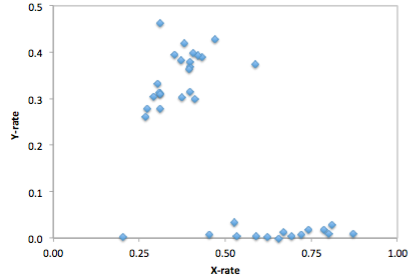
As you can see, in this case the relative Y chromosome coverage provides a much better separation of samples into (presumably) male and female, so here the authors used a relative y coverage of >0.2 to determine males, and <0.05 to determine females. Often, unfortunately, clustering is much less pronounced, and you will have to manually decide how to flag samples as “male”, “female” or “unknown”.
Nuclear contamination estimates in Males
Now that we have classified at least some samples as “probably male”, we can use their haploid X chromosome to estimate nuclear contamination. For this, we use the ANGSD-software. According to the ANGSD-Documentation, estimating X chromosome contamination from BAM files involves two steps.
The first step counts how often each of the four alleles is seen in variable sites in the X chromosome of a sample:
angsd -i $BAM -r X:5000000-154900000 -doCounts 1 -iCounts 1 -minMapQ 30 -minQ 30 -out $OUT
Here, I assume that the X chromosome is called X. If in your bam file it’s called chrX, you need to replace the region specification in the -r flag above. Note that the range 5Mb-154Mb is used in the example in the website, so I just copied it here. The $OUT file above actually denotes a filename-prefix, since there will be several output files from this command, which attach different file-endings after the given prefix.
To loop this command again over all samples, write a shell script as shown above, check the correct commands via an echo command and if they are correct, submit them using sbatch. My script looks like this:
#!/usr/bin/env bash

BAMDIR=/data/schiffels/MyProject/mergedBams.backup
OUTDIR=/data/schiffels/GAworkshop/xContamination
mkdir -p $OUTDIR

for SAMPLE in $(ls $BAMDIR); do
    BAM=$BAMDIR/$SAMPLE/$SAMPLE.mapped.sorted.rmdup.bam
    OUT=$OUTDIR/$SAMPLE.angsdCounts
    CMD="angsd -i $BAM -r X:5000000-154900000 -doCounts 1 -iCounts 1 -minMapQ 30 -minQ 30 -out $OUT"
    echo "$CMD"
    # sbatch -o $OUTDIR/$SAMPLE.angsdCounts.log --wrap="$CMD"
done
This should run very fast. Check whether the output folder is populated with non-empty files. You cannnot look at them easily because they are binary files.
The second step in ANGSD is the actual contamination estimation. Here is the command line recommended in the documentation:
/projects1/tools/angsd_0.910/misc/contamination -a $PREFIX.icnts.gz \
-h /projects1/tools/angsd_0.910/RES/HapMapChrX.gz 2> $OUT
Here, the executable is given with the full path because it is somewhat hidden. The $PREFIX variable should be replaced by the output-file prefix given in the previous (allele counting) command for the same sample. The HapMap file is provided by ANGSD and contains global allele frequency estimates used for the contamination calculation. Note that here we are not piping the standard out into the output file $OUT, but the standard error, indicated in bash via the special pipe 2>. The reason is that this ANGSD-program writes its results into the standard error rather than the standard output.
Again, you have to loop this through all samples like this:
#!/usr/bin/env bash

BAMDIR=/data/schiffels/MyProject/mergedBams.backup
OUTDIR=/data/schiffels/GAworkshop/xContamination
mkdir -p $OUTDIR

for SAMPLE in $(ls $BAMDIR); do
    PREFIX=$OUTDIR/$SAMPLE.angsdCounts
    OUT=$OUTDIR/$SAMPLE.xContamination.out
    HAPMAP=/projects1/tools/angsd_0.910/RES/HapMapChrX.gz
    CMD="/projects1/tools/angsd_0.910/misc/contamination -a $PREFIX.icnts.gz -h $HAPMAP 2> $OUT"
    echo "$CMD"
    # sbatch --mem=2000 -o $OUTDIR/$SAMPLE.xContamination.log --wrap="$CMD"
done
If this worked correctly, you should now have a contamination estimate for each sample. For a single sample, the output looks a bit messy, but the last line should read:
Method2: new_llh Version: MoM:0.072969 SE(MoM):5.964563e-02 ML:0.079651 SE(ML):7.892058e-16
This is the line indicating the contamination estimate using the “Methods of Moments” (MoM), and its standard error SE(MoM). You can grep all those lines:
adminschif@cdag1 /data/schiffels/GAworkshop/xContamination $ grep 'Method2: new_llh' *.out
JK2131udg.xContamination.out:Method2: new_llh Version: MoM:0.285843 SE(MoM):3.993658e-02 ML:0.281400 SE(ML):4.625781e-14
JK2132udg.xContamination.out:Method2: new_llh Version: MoM:0.133319 SE(MoM):9.339797e-02 ML:0.140492 SE(ML):0.000000e+00
JK2133udg.xContamination.out:Method2: new_llh Version: MoM:0.159191 SE(MoM):4.549252e-02 ML:0.160279 SE(ML):8.657070e-15
JK2134udg.xContamination.out:Method2: new_llh Version: MoM:-0.008918 SE(MoM):4.884321e-03 ML:-0.003724 SE(ML):9.784382e-17
...
You now want to include those results into your Excel table with the sex determination estimates. Copy them over to your laptop like shown above, in my case:
mkdir -p ~/Data/GAworkshop/contamination
scp adminschif@cdag1.cdag.shh.mpg.de:/data/schiffels/GAworkshop/xContamination/*.xContamination.out ~/Data/GAworkshop/contamination/
and you can now generate a simpler output using a little bash script like this:
#!/usr/bin/env bash

printf "SAMPLE\tCONTAM\tSE\n"
for FILENAME in $(ls ~/Data/GAworkshop/contamination/*.xContamination.out); do
    SAMPLE=$(basename $FILENAME .xContamination.out)
    CONTAM=$(grep 'Method2: new_llh' $FILENAME | cut -d' ' -f4 | cut -d: -f2)
    SE=$(grep 'Method2: new_llh' $FILENAME | cut -d' ' -f5 | cut -d: -f2)
    printf "$SAMPLE\t$CONTAM\t$SE\n"
done
If you run this, you may find that in some cases the output is empty, because angsd failed. You should then go back and check - for those samples - the *.log output from the contamination run above to see what was the reason for failure. In some cases, SLURM killed the job because it exceeded memory. You should then increase the memory set in the --mem flag in sbatch. In other cases, angsd failed for unknown reasons... nothing we can do about currently.
Finally, you can use this table, feed it into Excel and find male samples with low contamination to proceed with in the analysis.